ENDFACE TESTING
Made by Promet Optics

This is the 2nd of a 3 part post from the white paper entitled “Fiber Optic 3D Metrology”. We will define and lay out the necessity of measuring endface geometry as well as a conceptual overview of Michelson Interferometry, which is used to measure it.
Typically, a simple visual inspection using a hand-held microscope is used to look at the endface of a connector to check for contaminants and damage. However, using a microscope only tells part of the story. As seen in Figure 1, both connector ends look free from contaminants and damage which would lead the user to believe that both connectors are acceptable for use in a network.
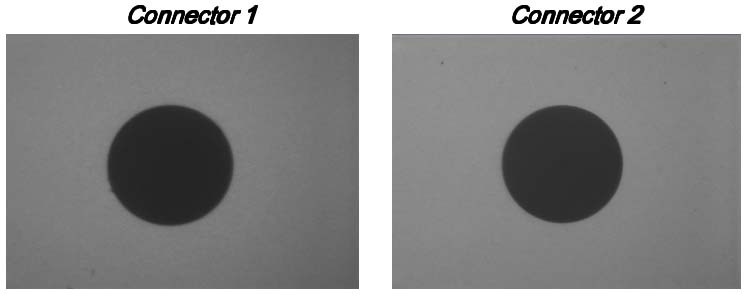
Fig. 1: Microscope image of connector endfaces
However, employing an interferometer designed specifically for connector endface measurement, such as PROMET’s FiBO®, the three-dimensional shape of the endface is revealed. The interference fringe images in Figure 2 suggest that the endface geometries of the two connectors are not the same.
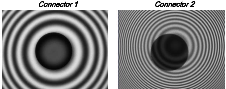
Fig. 2: Interference fringe image of connector endfaces
Taking interferometric measurements and generating the three-dimensional surface maps in Figure 3, clearly shows that the Connector 2 endface has an unacceptably small radius of curvature, only 3.5mm, while the Connector 1 endface has an acceptable radius of 14.0mm.
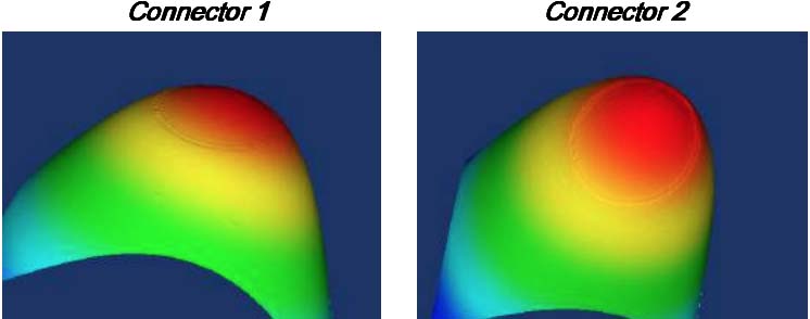
Fig. 3: Resulting three-dimensional maps
If Connector 2 is mated to a connector with correct endface geometry, unacceptable losses could result. In order to optimize network performance, connector endface geometries must be measured and controlled.
Read on to learn the basics of how interferometry works and how it can be used to measure the geometrical parameters of a connector endface.
Interferometry
In order to measure the three-dimensional parameters of a fiber optic connector endface, optical interferometry is typically used. Optical interferometry is a well known optical phenomenon that has found uses in inertial navigation, optical metrology, holography, astronomy, and many other fields. This section will describe the very basics of interferometry and how it can be used to generate fiber optic connector three-dimensional measurements.
Optical Interference
Optical interferometry is a non-contact measurement technique that relies on the interference between two beams of light. It is preferred over contact measurement methods which can damage the connector endface. Optical interference occurs when two coherent beams of light overlap. The wave nature of the two beams can be thought of as sine waves having a period the wavelength of the illuminating light. Where the two beams overlap, they can be added together using the property of superposition. When the peaks and valleys of the two sine waves line up perfectly, bright total constructive interference occurs. When the peaks of one sine wave line up perfectly with the valleys of the other sine wave, dark total destructive interference results. When the two sine waves are lined up in neither of the previous two scenarios, various levels of gray occur, depending on the amount of phase difference between the two sine waves.
The diagrams in Figure 4 show two interfering sine waves with varying amounts of phase difference between them and their sum. As the phase difference goes from 0 to 360 degrees, the results go from total constructive interference at 0 degrees, to total destructive interference at 180 degrees, and back to total constructive interference at 360 degrees.
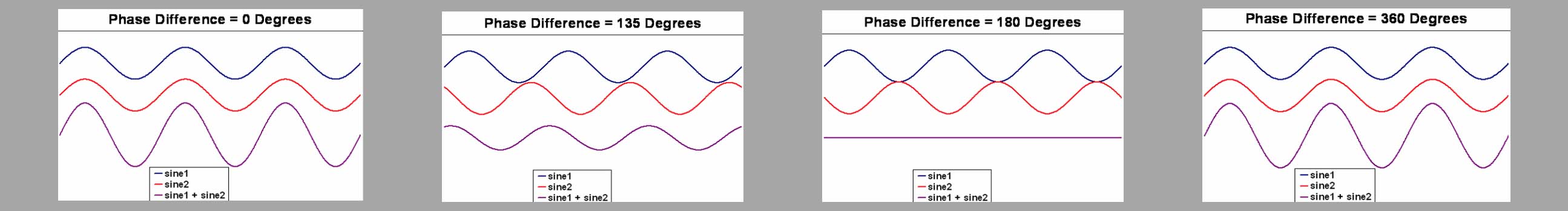
Fig. 4: Interference of two sine waves with 0 to 360 degrees phase difference
Michelson Interferometer
FiBO® is an example of a Michelson style interferometer, which forms interference fringes by dividing the illuminating light into two beams using a beamsplitter. The layout of a typical Michelson interferometer is depicted in Figure 6:
One beam bounces off of a reference mirror (orange beam) and the other beam is reflected from the connector endface (yellow beam). These beams are recombined by the beamsplitter and are imaged onto a camera (green beam). When overlapping parts of the two light beams travel distances that are multiples of the wavelength of the light, their electric fields line up and constructive interference occurs and a bright fringe is seen. When overlapping parts of the two beams travel distances that are odd multiples of half the wavelength of light, their electric fields are perfectly out of phase, and destructive interference occurs. Figure 7 shows an image with fringes that occur between a flat reference mirror and a spherically shaped connector endface. The black circle in the center is a 125 micron diameter fiber.
The circular fringes are like the contours of a topographical map showing where points of equal phase difference are occurring. The height difference between adjacent bright fringes corresponds to half the wavelength of light (approximately 0.32 microns).
Phase-Shifting Interferometry
A skilled operator can look at the fringes produced by a Michelson interferometer alone and get an idea of the three dimensional shape of the connector end. However, generating quantitative information is desirable to remove the user’s (in)experience from the equation and ensure objectivity. One of the most accurate techniques to obtain quantitative three-dimensional surface data is called phase-shifting interferometry. In this technique, the reference mirror of the Michelson interferometer is mounted on a piezoelectric actuator. The reference mirror is moved by this piezo by very precise amounts, which varies the phase difference between the two arms of the interferometer. Images are taken with a series of different phase amounts, typically 90 degrees between images (see Figure 8), and then are algebraically combined to obtain a phase map of the surface. There are different algorithms that have been developed to arrive at a phase map. This phase map is then converted to quantitative three-dimensional information.